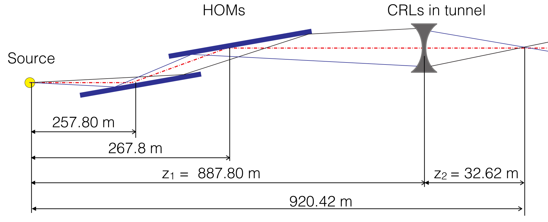
S1 SPB CRL simplified beamline
%matplotlib inline
from __future__ import absolute_import
from __future__ import division
from __future__ import print_function
from __future__ import unicode_literals
import os
import sys


# wpg_path = '/afs/desy.de/group/exfel/software/wpg/latest/' # DESY installation
wpg_path = os.path.join('..','..','..')
sys.path.insert(0, wpg_path)

import numpy as np
import pylab as plt


from wpg import Wavefront, Beamline
from wpg.optical_elements import Aperture, Drift, CRL, Empty, Use_PP
from wpg.generators import build_gauss_wavefront

from wpg.srwlib import srwl

from wpg.wpg_uti_exfl import calculate_theta_fwhm_cdr_s1
from wpg.wpg_uti_wf import calculate_fwhm, averaged_intensity, look_at_q_space, plot_t_wf
from wpg.wpg_uti_oe import show_transmission
from IPython.display import Image
Image(filename='CRL_1.png')
%%file bl_S1_SPB_CRL_simplified.py


def get_beamline():
    from wpg import Beamline
    from wpg.optical_elements import Aperture, Drift, CRL, Empty, Use_PP
    #S1 beamline layout
    ### Geometry ###
    src_to_hom1 = 257.8 # Distance source to HOM 1 [m]
    src_to_hom2 = 267.8 # Distance source to HOM 2 [m]
    src_to_crl = 887.8  # Distance source to CRL [m]
#     src_to_exp = 920.42 # Distance source to experiment [m]
    z0 = src_to_hom1

    # Drift to focus aperture
    #crl_to_exp_drift = Drift( src_to_exp - src_to_crl )
    z = 34.0
    #define distances, angles, etc
    #...
    #Incidence angle at HOM
    theta_om = 3.6e-3       # [rad]

    om_mirror_length = 0.8 # [m]
    om_clear_ap = om_mirror_length*theta_om


    #define the beamline:
    bl0 = Beamline()
    zoom=1

    # Define HOM1.
    aperture_x_to_y_ratio = 1
    hom1 = Aperture(shape='r',ap_or_ob='a',Dx=om_clear_ap,Dy=om_clear_ap/aperture_x_to_y_ratio)
    bl0.append( hom1, Use_PP(semi_analytical_treatment=0, zoom=zoom, sampling=zoom) )

    # Free space propagation from hom1 to hom2
    hom1_to_hom2_drift = Drift(src_to_hom2 - src_to_hom1); z0 = z0+(src_to_hom2 - src_to_hom1)
    bl0.append( hom1_to_hom2_drift, Use_PP(semi_analytical_treatment=0))


    # Define HOM2.
    zoom = 1.0
    hom2 = Aperture('r','a', om_clear_ap, om_clear_ap/aperture_x_to_y_ratio)
    bl0.append( hom2,  Use_PP(semi_analytical_treatment=0, zoom=zoom, sampling=zoom/0.75))

    #drift to CRL aperture
    hom2_to_crl_drift = Drift( src_to_crl - src_to_hom2 );z0 = z0+( src_to_crl - src_to_hom2 )
    #bl0.append( hom2_to_crl_drift, Use_PP(semi_analytical_treatment=0))
    bl0.append( hom2_to_crl_drift, Use_PP(semi_analytical_treatment=1))


    # Define CRL
    crl_focussing_plane = 3 # Both horizontal and vertical.
    crl_delta = 4.7177e-06 # Refractive index decrement (n = 1- delta - i*beta)
    crl_attenuation_length  = 6.3e-3    # Attenuation length [m], Henke data.
    crl_shape = 1         # Parabolic lenses
    crl_aperture = 5.0e-3 # [m]
    crl_curvature_radius = 5.8e-3 # [m]
    crl_number_of_lenses = 19
    crl_wall_thickness = 8.0e-5 # Thickness
    crl_center_horizontal_coordinate = 0.0
    crl_center_vertical_coordinate = 0.0
    crl_initial_photon_energy = 8.48e3 # [eV] ### OK ???
    crl_final_photon_energy = 8.52e3 # [eV]   ### OK ???

    crl = CRL( _foc_plane=crl_focussing_plane,
              _delta=crl_delta,
              _atten_len=crl_attenuation_length,
              _shape=crl_shape,
              _apert_h=crl_aperture,
              _apert_v=crl_aperture,
              _r_min=crl_curvature_radius,
              _n=crl_number_of_lenses,
              _wall_thick=crl_wall_thickness,
              _xc=crl_center_horizontal_coordinate,
              _yc=crl_center_vertical_coordinate,
              _void_cen_rad=None,
              _e_start=crl_initial_photon_energy,
              _e_fin=crl_final_photon_energy,
             )
    zoom=0.6

    bl0.append( crl, Use_PP(semi_analytical_treatment=1, zoom=zoom, sampling=zoom/0.1) )


    crl_to_exp_drift = Drift( z ); z0 = z0+z
    bl0.append( crl_to_exp_drift, Use_PP(semi_analytical_treatment=1, zoom=1, sampling=1))
#     bl0.append(Empty(),Use_PP(zoom=0.25, sampling=0.25))

    return bl0
Overwriting bl_S1_SPB_CRL_simplified.py
initial Gaussian wavefront
With the calculated beam parameters the initial wavefront is build with 400x400 data points and at distance of the first flat offset mirror at 257.8 m. For further propagation the built wavefront should be stored.
After plotting the wavefront the FWHM could be printed out and compared with Gaussian beam divergence value. #### Gaussian beam radius and size at distance \(z\) from the waist: \(\omega(z) = \omega_0*\sqrt{1+\left(\frac{z}{z_R}\right)^2}\), where \(\frac{1}{z_R} = \frac{\lambda}{\pi\omega_0^2}\)
Expected FWHM at first screen or focusing mirror: \(\theta_{FWHM}*z\)
src_to_hom1 = 257.8 # Distance source to HOM 1 [m]

# Central photon energy.
ekev = 8.5 # Energy [keV]

# Pulse parameters.
qnC = 0.5               # e-bunch charge, [nC]
pulse_duration = 9.e-15 # [s] <-is not used really, only ~coh time pulse duration has physical meaning
pulseEnergy = 1.5e-3    # total pulse energy, J
coh_time = 0.8e-15     # [s]<-should be SASE coherence time, then spectrum will be the same as for SASE
                       # check coherence time for 8 keV 0.5 nC SASE1

# Angular distribution
theta_fwhm = calculate_theta_fwhm_cdr_s1(ekev,qnC) # From tutorial
#theta_fwhm = 2.124e-6 # Beam divergence        # From Patrick's raytrace.

# Gaussian beam parameters
wlambda = 12.4*1e-10/ekev # wavelength
w0 = wlambda/(np.pi*theta_fwhm) # beam waist;
zR = (np.pi*w0**2)/wlambda # Rayleigh range
fwhm_at_zR = theta_fwhm*zR # FWHM at Rayleigh range
sigmaAmp = w0/(2*np.sqrt(np.log(2))) # sigma of amplitude

print('expected FWHM at distance {:.1f} m is {:.2f} mm'.format(src_to_hom1,theta_fwhm*src_to_hom1*1e3))

# expected beam radius at M1 position to get the range of the wavefront
sig_num = 5.5
range_xy = w0 * np.sqrt(1+(src_to_hom1/zR)**2) *sig_num;#print('range_xy at HOM1: {:.1f} mm'.format(range_xy*1e3))
fname = 'at_{:.0f}_m'.format(src_to_hom1)
expected FWHM at distance 257.8 m is 0.53 mm
bSaved=False
num_points = 400 #number of points
dx = 10.e-6; range_xy = dx*(num_points-1);#print('range_xy :', range_xy)
nslices = 20;

srwl_wf = build_gauss_wavefront(num_points, num_points, nslices, ekev, -range_xy/2, range_xy/2,
                                -range_xy/2, range_xy/2 ,coh_time/np.sqrt(2),
                                sigmaAmp, sigmaAmp, src_to_hom1,
                                pulseEn=pulseEnergy, pulseRange=8.)
wf = Wavefront(srwl_wf)
z0 = src_to_hom1
#defining name HDF5 file for storing wavefront
strOutInDataFolder = 'data_common'
#store wavefront to HDF5 file
if bSaved:
    wf.store_hdf5(fname+'.h5'); print('saving WF to %s' %fname+'.h5')

xx=calculate_fwhm(wf);
print('FWHM at distance {:.1f} m: {:.2f} x {:.2f} mm2'.format(z0,xx[u'fwhm_x']*1e3,xx[u'fwhm_y']*1e3));
FWHM at distance 257.8 m: 0.52 x 0.52 mm2
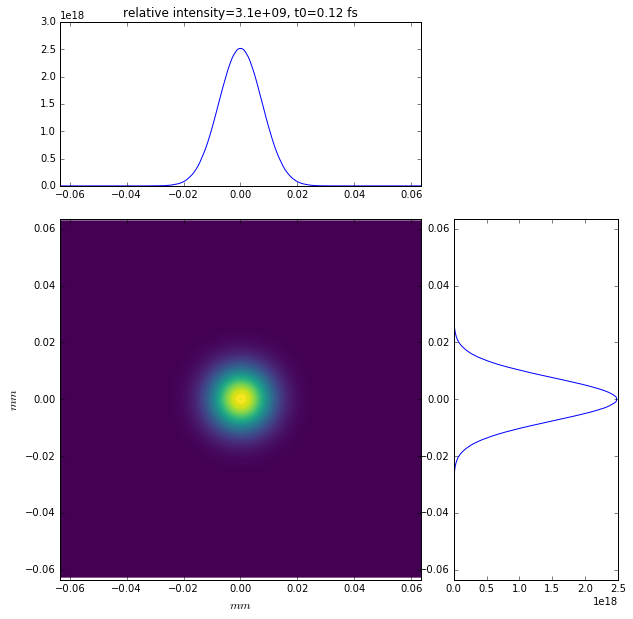
#input gaussian beam
print( 'dy {:.1f} um'.format((wf.params.Mesh.yMax-wf.params.Mesh.yMin)*1e6/(wf.params.Mesh.ny-1.)))
print( 'dx {:.1f} um'.format((wf.params.Mesh.xMax-wf.params.Mesh.xMin)*1e6/(wf.params.Mesh.nx-1.)))
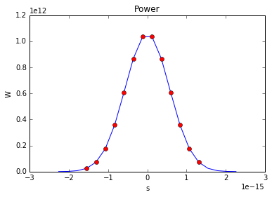
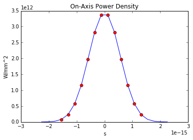
plot_t_wf(wf)
look_at_q_space(wf)
dy 10.0 um
dx 10.0 um
number of meaningful slices: 13
R-space
(400,) (400,)
Q-space
{'fwhm_y': 1.999254044117647e-06, 'fwhm_x': 1.999254044117647e-06}
Q-space
(400,) (400,)
#loading beamline from file
import imp
custom_beamline = imp.load_source('custom_beamline', 'bl_S1_SPB_CRL_simplified.py')
get_beamline = custom_beamline.get_beamline
bl = get_beamline()
print(bl)
Optical Element Setup: CRL Focal Length: 32.35296414510639 m
Optical Element: Aperture / Obstacle
Prop. parameters = [0, 0, 1.0, 0, 0, 1.0, 1.0, 1.0, 1.0, 0, 0, 0]
    Dx = 0.00288
    Dy = 0.00288
    ap_or_ob = a
    shape = r
    x = 0
    y = 0

Optical Element: Drift Space
Prop. parameters = [0, 0, 1.0, 0, 0, 1.0, 1.0, 1.0, 1.0, 0, 0, 0]
    L = 10.0
    treat = 0

Optical Element: Aperture / Obstacle
Prop. parameters = [0, 0, 1.0, 0, 0, 1.0, 1.3333333333333333, 1.0, 1.3333333333333333, 0, 0, 0]
    Dx = 0.00288
    Dy = 0.00288
    ap_or_ob = a
    shape = r
    x = 0
    y = 0

Optical Element: Drift Space
Prop. parameters = [0, 0, 1.0, 1, 0, 1.0, 1.0, 1.0, 1.0, 0, 0, 0]
    L = 620.0
    treat = 0

Optical Element: Transmission (generic)
Prop. parameters = [0, 0, 1.0, 1, 0, 0.6, 5.999999999999999, 0.6, 5.999999999999999, 0, 0, 0]
    Fx = 32.35296414510639
    Fy = 32.35296414510639
    arTr = array of size 2004002
    extTr = 1
    mesh = Radiation Mesh (Sampling)
            arSurf = None
            eFin = 8520.0
            eStart = 8480.0
            hvx = 1
            hvy = 0
            hvz = 0
            ne = 1
            nvx = 0
            nvy = 0
            nvz = 1
            nx = 1001
            ny = 1001
            xFin = 0.0027500000000000003
            xStart = -0.0027500000000000003
            yFin = 0.0027500000000000003
            yStart = -0.0027500000000000003
            zStart = 0


Optical Element: Drift Space
Prop. parameters = [0, 0, 1.0, 1, 0, 1.0, 1.0, 1.0, 1.0, 0, 0, 0]
    L = 34.0
    treat = 0
#propagated gaussian beam
srwl.SetRepresElecField(wf._srwl_wf, 'f') # <---- switch to frequency domain
bl.propagate(wf)
srwl.SetRepresElecField(wf._srwl_wf, 't')
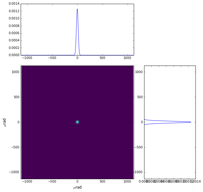
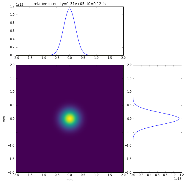
print('FWHM after CRLs:');print(calculate_fwhm(wf))
print('FWHM at distance {:.1f} m:'.format(wf.params.Mesh.zCoord));print(calculate_fwhm(wf))
plot_t_wf(wf)
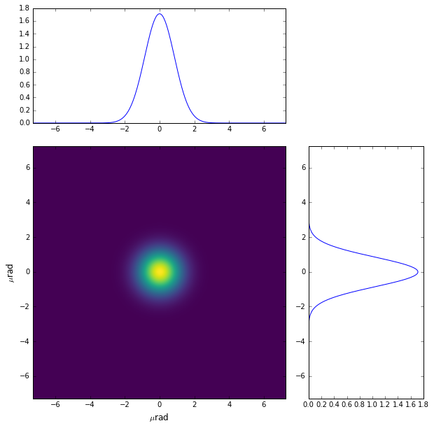
look_at_q_space(wf)
FWHM after CRLs:
{'fwhm_y': 1.779350912766013e-05, 'fwhm_x': 1.7897682395761173e-05}
FWHM at distance 921.8 m:
{'fwhm_y': 1.779350912766013e-05, 'fwhm_x': 1.7897682395761173e-05}
number of meaningful slices: 13
R-space
(1944,) (1944,)
Q-space
{'fwhm_y': 4.298910472684863e-05, 'fwhm_x': 4.242918502417042e-05}
Q-space
(1944,) (1944,)